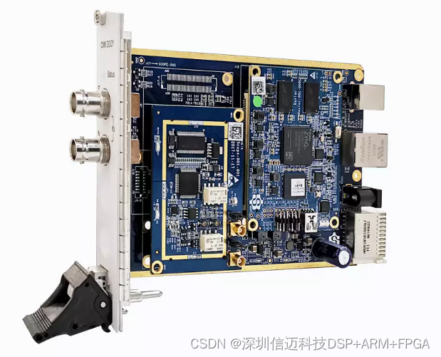
Plug-in Instrument Module: Oscilloscope Module (Plug-in)

Sienovo's plug-in oscilloscope module brings bench-grade waveform capture directly into a modular instrument chassis, giving embedded and power engineers a portable, software-driven alternative to a standalone scope. This post walks through the module's key specifications, explains the tradeoffs between the single-channel and dual-channel configurations, and covers the practical measurement scenarios each variant is best suited for.

What Is a Plug-in Oscilloscope Module?

Plug-in instrument modules follow the same philosophy as PXI and VXI: instead of a rack of dedicated benchtop instruments, a single chassis hosts interchangeable function-specific cards. The oscilloscope module described here occupies one slot and connects to the host system over a high-speed backplane interface. Because the digitiser, front-end conditioning, and signal path are all self-contained on the plug-in card, you get repeatable, calibrated measurements without the setup overhead of a full benchtop scope.

This particular module ships in two hardware variants — a single-channel (1×) version and a dual-channel (2×) version — each tuned for different application priorities.

Specifications at a Glance

| Parameter | 1× (Single-Channel) | 2× (Dual-Channel) | |---|---|---| | ADC Resolution | 12 bits | 12 bits | | Sampling Rate | 40 MSPS | 125 MSPS | | Bandwidth | 18 MHz | 30 MHz | | Input Range | ±1 V / ±10 V | ±0.9 V | | Input Impedance | Hi-Z, 1 MΩ | 1 MΩ | | Coupling | AC/DC | DC | | Measurement Resolution | 0.48 mV (±1 V range) / 4.8 mV (±10 V range) | 0.2 mV | | Measurement Accuracy (±1 V) | ±(0.1% of Reading + 0.01% of F.S.) | ±(0.1% of Reading + 0.1% of F.S.) | | Measurement Accuracy (±10 V) | ±(0.1% of Reading + 0.07% of F.S.) | — |

Single-Channel vs. Dual-Channel: Choosing the Right Variant

Single-Channel (1×): Wide Dynamic Range, High Accuracy

The 1× module is the better choice when you need to cover a wide voltage swing. Its dual input range — ±1 V and ±10 V — lets you work with everything from millivolt-level signal traces to 20 V peak-to-peak power rails without re-patching. Switching to the ±10 V range moves measurement resolution to 4.8 mV, which remains adequate for most power-supply characterisation tasks.

Accuracy on the narrow ±1 V range is impressive: the floor term is only 0.01% of full scale, which translates to roughly ±0.1 mV of offset error on top of the ±0.1%-of-reading gain error. That makes this variant appropriate for precision analogue measurements where absolute voltage matters, not just waveform shape.

The tradeoff is sampling rate: 40 MSPS gives a Nyquist limit of 20 MHz, consistent with the 18 MHz specified bandwidth. You will not capture fast transients above that frequency with this card.

Dual-Channel (2×): Higher Speed, Better Resolution

The 2× module runs at 125 MSPS, nearly three times the single-channel rate, and extends bandwidth to 30 MHz. Measurement resolution improves to 0.2 mV — finer than the single-channel's ±1 V resolution — which is useful when you need to resolve small differential signals between two related nodes simultaneously.

The narrower ±0.9 V input range and DC-only coupling mean the 2× variant is optimised for low-voltage digital or RF-adjacent signals rather than wide-range power measurements. Because AC coupling is absent, you must account for any DC offset in your measurement setup manually.

Practical Measurement Use Cases

Power-Up Timing Measurement

During board bring-up, verifying that power rails sequence correctly is critical. A misordered power-on sequence can latch up ICs or cause undefined boot states. With the dual-channel variant you can probe two rails simultaneously and measure the time interval between their rising edges directly from the captured waveforms, giving you a precise timing margin relative to datasheet requirements.

Waveform Analysis: Period, Amplitude, and Anomalies

Once a system is running, the module can continuously capture waveforms and compute period, frequency, and amplitude statistics. More importantly, it can flag anomalies — glitches, runt pulses, or unexpected frequency deviations — that only appear sporadically and would be missed by a DMM or a slow logger.

Power Supply Ripple and Noise Analysis

Switching converters generate ripple at the switching frequency and harmonics, plus broadband noise from diode recovery and EMI coupling. The module's 12-bit resolution (versus the 8 bits typical of general-purpose oscilloscopes) gives you roughly 48 dB of dynamic range, letting you resolve millivolt-level ripple on top of a multi-volt DC rail without rescaling.

Signal Template Comparison

Template (mask) testing overlays a captured "golden" waveform boundary on live captures and flags any sample that falls outside the envelope. This is a standard production-test technique for verifying that a circuit's output waveform stays within specification across units or over temperature without requiring manual inspection of every acquisition.

Wireless Charging Signal Demodulation

Wireless power transfer protocols such as Qi encode data by modulating the amplitude or frequency of the power carrier. The module's combination of sufficient bandwidth, 12-bit resolution, and DC coupling makes it possible to demodulate this signal in software — capturing the carrier envelope, applying digital filtering, and decoding the embedded communication frames — without a separate communications analyser.

Integration Considerations

Because this is a plug-in module, the actual trigger, timebase, and data transfer logic live in the host chassis firmware and software. When evaluating acquisition throughput in a real application, account for the backplane transfer bandwidth: at 125 MSPS with 12-bit samples, the raw data rate is 1.5 Gbit/s per channel, so most practical deployments use hardware decimation, hardware triggering with pre/post-trigger buffers, or segmented-memory acquisition to capture only the intervals of interest rather than streaming continuously.

For FPGA-based chassis platforms, the ADC data typically arrives over an LVDS bus and feeds directly into a capture buffer in block RAM, with a soft trigger state machine controlling when samples are committed to host memory. This architecture keeps trigger latency deterministic and independent of host OS scheduling jitter.